 |
We gathered a large set of programs from public sources and defined a learning problem with two classes: malicious and benign executables. Each example in the data set is a Windows or MS-DOS format executable, although the framework we present is applicable to other formats. To standardize our data-set, we used MacAfee's [6] virus scanner and labeled our programs as either malicious or benign executables.
We split the dataset into two subsets: the training set and the test set. The data mining algorithms used the training set while generating the rule sets, and after training we used a test set to test the accuracy of the classifiers on a set of unseen examples.
The data set consisted of a total of 4,301 programs split into 3,301 malicious binaries and 1,000 benign programs. The malicious binaries consisted of viruses, Trojans, and cracker/network tools. There were no duplicate programs in the data set and every example in the set is labeled either malicious or benign by the commercial virus scanner. All labels are assumed to be correct.
All programs were gathered either from FTP sites, or personal computers in the Data Mining Lab at Columbia University. To obtain the dataset please contact us through our website http://www.cs.columbia.edu/ids/mef/.
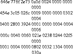
We statically extracted byte sequence features from each binary example for the learning algorithms. Features in a data mining framework are properties extracted from each example in the data set, such as byte sequences, that a classifier uses to generate detection models. These features are then used by the algorithms to generate detection models. We used hexdump [7], an open source tool that transforms binary files into hexadecimal files. After we generated the hexdumps we produced features in the form displayed in Figure 1 where each line represents a short sequence of machine code instructions.
The classifier we incorporated into Procmail was a Naive Bayes classifier [1]. A naive Bayes classifier computes the likelihood that a program is malicious given the features that are contained in the program. We assumed that there were similar byte sequences in malicious executables that differentiated them from benign programs, and the class of benign programs had similar sequences that differentiated them from the malicious executables.
The model output by the naive Bayes algorithm labels examples based on the byte strings that they contain. For instance, if a program contained a significant number of malicious byte sequences and a few or no benign sequences, then it labels that binary as malicious. Likewise, a binary that was composed of many benign features and a smaller number of malicious features is labeled benign by the system.
The naive Bayes algorithm computed the probability that a given feature was malicious, and the probability that a feature was benign by computing statistics on the set of training data. Then to predict whether a binary, or collection of hex strings was malicious or benign, those probabilities were computed for each hex string in the binary, and then the Naive Bayes independence assumption was used. The independence assumption was applied in order to efficiently compute the probability that a binary was malicious and the probability that the binary was benign.
One draw back of the naive Bayes method was that it requires more than 1 GB of RAM to generate its detection model. To make the algorithm more efficient we divided the problem into smaller pieces that would fit in memory and generated a classifier for each of the subproblems. The subproblem was to classify based on every 16 subsets of the data organized according to the first letter of the hex string.
For this we trained sixteen Naive Bayes classifiers so that all hex strings were trained on. For example, one classifier trained on all hex strings starting with an ``A'', and another on all hex strings starting with a ``0''. This was done 16 times and then a voting algorithm was then used to combine their outputs.
A more thorough description along with an example, can be found in a companion paper [10].
To compare our results with traditional methods we implemented a signature based method. First, we calculated the byte-sequences that were only found in the malicious executable class. These byte-sequences were then concatenated together to make a unique signature for each malicious executable example. Thus each malicious executable signature contained only byte-sequences found in the malicious executable class. To make the signature unique, the byte-sequences found in each example were concatenated together to form one signature. This was done because a byte-sequence that was only found in one class during training could possibly be found in the other class during testing [4], and lead to false positives when deployed.
The virus scanner that we used to label the data set contained signatures for every malicious example in our data set, so it was necessary to implement a similar signature-based method. This was done to compare the two algorithms' accuracy in detecting new malicious executables. In our tests the signature-based algorithm was only allowed to generate signatures for the same set of training data that the data mining method used. This allowed the two methods to be fairly compared. The comparison was made by testing the two methods on a set of binaries not contained in the training set.
To quantify the performance of our method we computed statistics on the preformance of the data mining-based method versus the signature-based method. We are interested in four quantities in the experiments. They are the counts for true positives, true negatives, false positives, and false negatives. A true positive, TP, is an malicious example that is correctly tagged as malicious, and a true negative, TN, is a benign example that is correctly classified as benign. A false positive, FP, is a benign program that has been mislabeled by an algorithm as malicious, while a false negative, FN, is a malicious executable that has been mis-classified as a benign program.
The overall accuracy of the algorithm is calculated as the number of programs the system classified correctly divided by the total number of binaries tested. The detection rate is the number of malicious binaries correctly classified divided by the total number of malicious programs tested.
We estimated our results for detecting new executables by using 5-fold cross validation [5]. Cross validation is the standard method to estimate the performance of predictions over unseen data. For each set of binary profiles we partitioned the data into five equal size partitions. We used four of the partitions for training a model and then evaluated that model on the remaining partition. Then we repeated the process five times leaving out a different partition for testing each time. This gave us a reliable measure of our method's accuracy on unseen data. We averaged the results of these five tests to obtain a measure of how the algorithm performs in detecting new malicious executables.
Table 1 displays the results. The data mining algorithm had the highest detection rate, 97.76% compared with the signature based method's detection rate of 33.96%. Along with the higher detection rate the data mining method had a higher overall accuracy, 96.88% vs. 49.31%. The false positive rate at 6.01% though was higher than the signature based method, 0%.
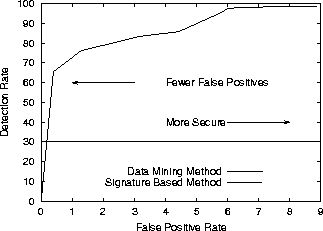
Figure 2 displays the plot of the detection rate vs. false positive rate using Receiver Operation Characteristic curves [13]. Receiver Operating Characteristic (ROC) curves are a way of visualizing the trade-offs between detection and false positive rates. In this instance, the ROC curve show how the data mining method can be configured for different environments. For a false positive rate less than or equal to 1% the detection rate would be greater than 70%, and for a false positive rate greater than 8% the detection rate would be greater than 99%.
|
We also evaluated the performance of the models in detecting known executables. For this task, the algorithms generated detection models for the entire set of data. Their performance was then evaluated by testing the models on the same training set.
|
As shown in Table 2, both methods detected over 99% of known executables. The data mining algorithm detected 99.87% of the malicious examples and misclassified 2% of the benign binaries as malicious. However, we have the signatures for the binaries that the data mining algorithm misclassified, and the algorithm can include those signatures in the detection model without lowering accuracy of the algorithm in detecting unknown binaries. After the signatures for the executables that were misclassified during training had been generated and included in the detection model, the data mining model had a 100% accuracy rate when tested on known executables.
 |