Versatile File System Tracing with Tracefs

A Thesis Presented
by
Akshat Aranya
to
The Graduate School
in Partial Fulfillment of the
Requirements
for the Degree of

Master of Science
in
Computer Science

Stony Brook University

Technical Report FSL-04-05
August 2004

Abstract of the Thesis
Versatile File System Tracing with Tracefs
by
Akshat Aranya
Master of Science
in
Computer Science
Stony Brook University
2004

File system traces have been used for years to analyze user behavior and system software behavior, leading to advances in file system and storage technologies. Existing traces, however, are difficult to use because they were captured for a specific use and cannot be changed, they often miss vital information for others to use, they become stale as time goes by, and they cannot be easily distributed due to user privacy concerns. Other forms of traces (block level, NFS level, or system-call level) all contain one or more deficiencies, limiting their usefulness to a wider range of studies.

We developed Tracefs, a thin stackable file system for capturing file system traces in a portable manner. Tracefs can capture uniform traces for any file system, without modifying the file systems being traced. Tracefs can capture traces at various degrees of granularity: by users, groups, processes, files and file names, file operations, and more; it can transform trace data into aggregate counters, compressed, checksummed, encrypted, or anonymized streams; and it can buffer and direct the resulting data to various destinations (e.g., sockets, disks, etc.). Our modular and extensible design allows for uses beyond traditional file system traces: Tracefs can wrap around other file systems for debugging as well as for feeding user activity data into an Intrusion Detection System. We have implemented and evaluated a prototype Tracefs on Linux. Our evaluation shows a highly versatile system with small overheads.

To Mummy, Daddy, and Rolee

1 Introduction
2 Design
    2.1 Component Architecture
    2.2 Input Filters
    2.3 Assembly Drivers
    2.4 Output Filters
    2.5 Output Drivers
    2.6 Trace Structure
    2.7 Versioning
    2.8 Anonymization
    2.9 Replaying Traces
    2.10 Usage
3 Implementation
    3.1 System call based filtering
    3.2 File name based filtering
    3.3 Asynchronous filter
4 Evaluation
    4.1 Configurations
    4.2 Workloads
    4.3 Am-Utils Results
    4.4 Postmark Results
    4.5 Trace File Sizes and Creation Rates
    4.6 Effect of Asynchronous Writes
    4.7 Multi-Process Scalability
    4.8 Anonymization Results
5 Related Work
6 Conclusions
    6.1 Future Work

List of Figures

    2.1 Architecture of Tracefs as a stackable file system
    2.2 Architecture of a Tracefs tracer
    2.3 Directed acyclic graph representing a trace condition
    2.4 BNF syntax of a trace file
    2.5 An example of a trace message
    3.1 The file name cache
    3.2 The asynchronous filter
    4.1 Execution times for an Am-Utils build
    4.2 Execution times for Postmark
    4.3 Trace file sizes and creation rates
    4.4 Performance of the asynchronous output filter
    4.5 Performance of a multithreaded application
    4.6 Trace file anonymization rates and file sizes

List of Tables

4.1 File system and asynchronous filter configurations
\LARGE{{Acknowledgments}}

Acknowledgments

I would like to thank my adviser, Dr. Erez Zadok, for his ideas, help, and encouragement that made this project possible. His guidance made my time at the FSL an excellent learning experience. I would also like to thank Dr. Tzi-cker Chiueh and Dr. R. Sekar for being on my committee and providing me with valuable inputs and comments. Charles Wright for his ideas and excellent C skills that helped me code my way out of a paper bag on many occasions. Nikolai Joukov for his contribution to trace replaying and the aggregate driver. Kiran-Kumar Muniswamy-Reddy for his help with benchmarking for the FAST submissions. Sean Callanan and Avishay Traeger for endless rounds of Crack Attack and Frozen Bubble that helped me keep sane. I would also like to thank the FAST community for their valuable feedback. Finally, a special thanks to Linus Torvalds and his band of geeks for providing me and the rest of the world an excellent platform to work on and tinker with.

This work was partially made possible by an NSF CAREER award EIA-0133589, NSF award CCR-0310493, and HP/Intel gifts numbers 87128 and 88415.1.

Chapter 1
Introduction

File system traces have been used in the past to analyze the user access patterns and file system software performance. Studies using those traces helped the community devise better software and hardware to accommodate ever-changing computing needs [15,1,19]. For example, traces can be used to determine dynamic access patterns of file systems such as the rate of file creation, the distribution of read and write operations, file sizes, file lifetimes, the frequency of each file system operation, etc. The information collected through traces is useful to determine file system bottlenecks. It can help identify typical usage patterns that can be optimized and provide valuable data for improving performance.

Although the primary use of traces had been for file system performance studies [19], two other uses exist: security and debugging. First, file system tracing is useful for security and auditing. Monitoring file system operations can help detect intrusions and assess the damage. Tracing can be conducted file system wide or based on a suspected user, program, or process. Also, file system tracing has the potential for use in computer forensics-to roll back and replay the traced operations, or to revert a file system to a state prior to an attack.

Second, file system tracing is useful for debugging other file systems. A fine-grained tracing facility can allow a file system developer to locate bugs and points of failure. For example, a developer may want to trace just one system call made into the file system, or all calls made by a particular process, or turn tracing on and off dynamically at critical times. A tracing file system that can be easily layered or stacked on top of another file system is particularly suitable for debugging as it requires no modification to the file system or the OS.

Previous tracing systems were customized for a single study [15,19]. These systems were built either in an ad-hoc manner, or were not well documented in research texts. Their emphasis was on studying the characteristics of file system operations and not on developing a systematic or reusable infrastructure for tracing. After such studies were published, the traces would sometimes be released. Often, the traces excluded useful information for others conducting new studies; information excluded could concern the initial state of the machines or hardware on which the traces were collected, some file system operations and their arguments, pathnames, and more. For example, block-level traces often lack specific information about file system operations and user activity. NFS-level traces lack information about the state of the applications and users running on the clients, or the servers' state. System-call level traces often miss information about how system call activity is translated into multiple actions in the lower layers of the OS. System-call traces also cannot work on NFS servers where no system call activity is seen by the server.

To illustrate typical problems when using past traces, we describe our own experiences. In the past two years, we conducted a study comparing the growth rate of disk sizes to the growth rate of users' disk space consumption; we required information about the growth rate of various types of files. To determine file types, we used the files' extensions [6]. The traces we were able to access proved unsuitable for our needs. The Sprite [1] and BSD [15] traces were too old to be meaningful for today's fast-changing systems. These two also did not include the full file's pathname or size. The "Labyrinth" and "Lair" passive NFS traces (which were not available at the time we conducted our study) only show patterns as seen over the NFS protocol, lacking client and server information [5]. Eventually, we found two traces which, when combined, could provide us with the data required: the SEER [11] and Roselli [19] traces. Even then, we had to contact the authors of those traces to request additional information about the systems on which those traces were taken. Next, we attempted to draw conclusions from the combination of the two distinct traces, a less-than-ideal situation for precise studies. Finally, to verify our conclusions, we had to capture our own traces and correlate them with past traces. Our experience is not uncommon: much time is wasted because available traces are unsuitable for the tasks at hand.

For traces to be useful for more than one study, they should include all information that could be necessary even years later. To be flexible, the tracing system should allow traces to be captured based on a wide range of fine-grained conditions. To be efficient in time and space, the system should trace only that which is desired, support buffering and compression, and more. To be secure, the trace system should support strong encryption and powerful anonymization. We have designed and implemented such a system, called Tracefs.

Tracefs uses a highly flexible and composable set of modules. Input filters can efficiently determine what to trace by users, groups, processes, sessions, file system operations, file names and attributes, and more. Output filters control trace data manipulations such as encryption, compression, buffering, checksumming-as well as aggregation operators that count frequencies of traced operations. Output drivers determine the amount of buffering to use and where the trace data stream should be directed: a raw device, a file, or a local or remote socket. The traces are portable and self-describing to preserve their usefulness in the future. A set of user-level tools can anonymize selective parts of a trace with encryption keys that can unlock desired subsets of anonymized data. Finally, our design decomposes the various components of the system in an extensible manner, to allow others to write additional input or output filters and drivers.

We chose a stackable file system implementation for Tracefs because it requires no changes to the operating system or the file systems being traced. A stackable file system can capture traces with the same ease whether running on individual clients' local file systems (e.g., Ext2 or FFS), on network file system mounts (e.g., NFS or SMBFS), or even directly on NFS file servers.

We developed a prototype of the Tracefs system on Linux. Our evaluation shows negligible time overheads for moderate levels of tracing. Tracefs demonstrates an overhead of less than 2% for normal user operations and 6% for an I/O-intensive workload.

The rest of the document is organized as follows. Chapter 2 describes the design of Tracefs. Chapter 3 discusses interesting implementation aspects. Chapter 4 presents an evaluation of Tracefs. Chapter 5 surveys related work. We conclude in Chapter 6 and discuss future directions.

Chapter 2
Design

We considered the following six design goals:

Flexibility Flexibility is the most important consideration for a tracing file system like Tracefs. Traditionally, tracing systems have either collected large amounts of traces that are cumbersome to store and parse or were focused at specific areas of study that make them less useful to other studies. We designed Tracefs to support different combinations of traced operations, verbosity of tracing, the trace destination, and security and performance features.
Performance It is essential that tracing does not incur too much performance overhead. Tracing is inherently an expensive operation, since it requires disk or network I/O. When designing tracing mechanisms, tradeoffs have to be made between performance and functionality. In our design, we addressed performance issues through buffering and provisions for limiting the data traced to exactly that which is relevant to each study.
Convenience of Analysis We designed Tracefs to use a simple binary format for generated traces. The traces are self-contained, i.e., they incorporate information about how the trace data is to be parsed and interpreted.
Security One of the uses for a tracing file system is to monitor malicious activity on a system. Hence, it is essential that the generated traces should be protected from attacks or subversion. We incorporated encryption and keyed checksums to provide strong security.
Privacy Public distribution of traces raises concerns about privacy since traces may contain personal information. Such information cannot simply be removed from traces since it is required for correlation. To address privacy concerns, we designed our system to anonymize traces while still retaining information required for correlation. Data fields in traces can be selectively anonymized, providing flexibility in choosing the parts of the traces that need to be anonymized.
Portability We achieved portability through the use of a stackable file system that is available on multiple platforms [22]. A stackable file system allows us to easily trace any underlying file system. Since Tracefs is implemented as a kernel module, no kernel modifications are required to enable tracing.

In Section 2.1 we describe the component architecture of Tracefs, and in Sections 2.2-2.5 we discuss each component in detail. In Section 2.6 we describe the trace file structure. In Section 2.8 we describe how traces are anonymized. In Section 2.10 we discuss usage scenarios.

2.1 Component Architecture

Tracefs is implemented as a stackable file system that can be stacked on top of any underlying file system. Figure 2.1 shows that Tracefs is a thin layer between the Virtual File System (VFS) and any other file system. File-system-related system calls invoke VFS calls which in turn invoke an underlying file system. When Tracefs is stacked on top of another file system, the VFS calls are intercepted by Tracefs before being passed to the underlying file system. Before invoking the underlying file system, Tracefs calls hooks into one or more tracers that trace the operation. Another hook is called at the end of the operation to trace the return value.

Figure 2.1: Architecture of Tracefs as a stackable file system. Tracefs intercepts operations and invokes hooks into one or more tracers before passing the operations to the underlying file system.

The use of stacking has several inherent advantages for tracing. Tracefs can be used to trace any file system. Moreover, memory-mapped I/O can only be traced at the file-system level. It is also more natural to study file system characteristics in terms of file system operations instead of system calls. Finally, server-side operations of network file systems are performed directly in the kernel, not through system calls.

Figure 2.2: Architecture for a Tracefs tracer. Assembly drivers generate a trace stream that is transformed by output filters before being written out by an output driver. An optional asynchronous filter buffers the trace stream that is processed by a separate kernel thread.

Figure 2.2 depicts the high level architecture of our tracing infrastructure. It consists of four major components: input filters, assembly drivers, output filters, and output drivers. Input filters are invoked using hooks from the file system layer. Input filters determine which operations to trace. Assembly drivers convert a traced operation and its parameters into a stream format. Output filters perform a series of stream transformations like encryption, compression, etc. Output drivers write the trace stream out from the kernel to an external entity, like a file or a socket.

A combination of an input filter, assembly drivers, output filters, and an output driver defines a tracer. Tracefs supports multiple tracers which makes it possible to trace the same system simultaneously under different trace configurations.

We have emphasized simplicity and extensibility in designing interfaces for assembly drivers, output filters, and output drivers. Each component has a well-defined API. The APIs can be used to extend the functionality of Tracefs. Writing custom drivers requires little knowledge of kernel programming or file system internals. An output driver or output filter defines five operations: initialize, release, write, flush, and get the preferred block size. An assembly driver requires the implementation of pre-call and post-call stubs for every VFS operation of interest. Including initialization and cleanup, an assembly driver can have up to 74 operations on Linux. Pre-call methods invoke the assembly driver before the actual operation is passed to the lower-level file system; post-call methods invoke the assembly driver after the call to the lower-level file system. For example, an assembly driver that is interested in counting the frequency of file creation and deletion need only implement two methods: CREATE and UNLINK. Custom drivers can be plugged into the existing infrastructure easily.

2.2 Input Filters

We use input filters to specify an expression that determines what operations are traced. For every file system operation, the expression is evaluated to determine if the operation needs to be traced. The user can specify arbitrary boolean expressions built from a set of basic predicates, such as UID, GID, PID, session ID, process name, file name, VFS operation type, system call name, etc. Input filters provide a flexible mechanism for generating specific traces based on the user's requirements.

An input filter is implemented as an in-kernel directed acyclic graph (DAG) that represents a boolean expression. We adapted the popular and efficient code for representing expressions from the Berkeley Packet Filter [12] and the PCAP library [9]. We evaluate an input filter against file system objects that were passed as parameters to the call and the current process's task structure. Fields in these structures define the tracing context for evaluating the truth value of the trace expression.

Figure 2.3: Directed acyclic graph representing the trace condition:

Figure 2.3 shows an example of one such expression and its DAG representation. Each non-terminal vertex in the graph represents a simple predicate, and has two outgoing edges labeled TRUE and FALSE. The graph has two terminal vertices representing the final result of the evaluation. Evaluation starts at the root vertex. At each step, the predicate of the vertex is evaluated, and one of the two outgoing edges is taken based on the result of the evaluation. This procedure is repeated until the graph traversal reaches either of the two terminal vertices.

We chose this approach over a standard tree representation since it is more compact and allows for a simple traversal from the start to a terminal vertex, instead of recursion or complex threaded traversal of trees. It also enables sharing of nodes [12].

To set up tracing, the DAG is constructed in user space and then passed to the kernel using an array. The kernel validates all the data fields, and verifies that the DAG does not contain any cycles. This way the kernel does not need to parse text expressions or construct graphs.

2.3 Assembly Drivers

Once the input filter has determined that a certain operation should be traced, the filter passes the corresponding VFS objects to a series of assembly drivers that determine the content of generated traces. An assembly driver is invoked through a well-defined interface that makes it easy to chain multiple assembly drivers together. We describe two assembly drivers: stream and aggregate.

Stream driver The stream driver is the default assembly driver. It converts the fields of VFS objects into a stream format. The stream driver generates one message for each logged file system operation. We describe the stream format in Section 2.6. The stream driver has various verbosity options that determine how much information is logged. Verbosity options allow the user to choose any combination of the following:

Fields of VFS objects like dentry, inode, or file, e.g., inode number, link count, and size.
Return values
Timestamps with second or microsecond resolution
Checksum for read and write data
Data in read and write operations
Process ID, session ID, process group ID
User ID, group ID
Process name
System call number
File name, file extension

Aggregate driver

One of the popular applications of tracing is to collect statistical distributions of operations, instead of actually logging each operation [19,1]. This has been traditionally performed by post-processing vast amounts of trace data and tallying the number of times each operation was invoked. It is wasteful to log each operation and its parameters since most of the information is discarded in post-processing.

For such applications, we have developed an aggregate driver that keeps track of the number of calls made during a tracing session and records the values at the end of the session. The aggregate driver also allows the user to determine per-operation execution times with a high precision. To achieve this, the aggregate driver uses a special hardware register that maintains a high-precision clock based on the CPU clock tick. The aggregate driver classifies the execution times into a set of geometrically-distributed buckets.

The aggregate driver provides an easy and efficient mechanism for extracting detailed information about operation execution times and the distribution of operations. The aggregate driver can be used in conjunction with input filters to determine specific statistical properties of file system operations; for example, to determine the access patterns of individual users.

2.4 Output Filters

Assembly drivers generate a stream of output and feed it to the first of a series of output filters. Output filters perform operations on a stream of bytes and have no knowledge about VFS objects or the trace file format. Each filter transforms the input stream and feeds it to the next filter in the chain. Output filters provide added functionality such as encryption, compression, and checksum calculation. During trace setup, the user can specify the output filters and their order. The filters can be inserted in any order as they are stream based. The last output filter in the chain feeds the trace stream to an output driver that writes the trace stream to the destination.

Each output filter maintains a default block size of 4KB. We chose a 4KB default, since it is the page size on most systems and it is a reasonably small unit of operation. However, the output filters are designed to operate on streams, therefore, the block sizes can be different for each output filter. The block size can be configured during trace setup.

We now describe four output filters: checksum, compression, encryption, and the asynchronous filter.

Checksum filter A checksum filter is used to verify the integrity of traces. It calculates a block-by-block HMAC-MD5 [18] digest and writes it at the end of each block. It uses a default block size of 4KB that can be overridden. The block size determines how frequently checksums are generated, and therefore, how much overhead checksumming has for the size of the trace file. Each block is also numbered with a sequence number that is included in the digest calculation, so that modification of traces by removal or reordering of blocks can be detected. Each trace file also uses a randomly-generated serial number that is included in each block so that a block in one trace file cannot be replaced with a block with the same sequence number from another file.

A checksum filter ensures that trace files are protected against malicious modifications. Also, since each block has its own digest, we can verify the integrity of each block separately. Even if a few blocks are modified, the unmodified blocks can still be trusted.

Compression filter Traces often contain repeated information. For example, the logged PID, UID, and GID are repeated for each operation performed by a process. Also, the meta-data of the traces, like message identifiers and argument identifiers, is often repeated. As a result, traces lend themselves well to compression.

The compression filter compresses trace data on-the-fly. Compression introduces additional overheads in terms of CPU usage, but it provides considerable savings in terms of I/O and storage space. The compression filter can be used when the size of traces needs to be kept small, or when I/O overheads are large, for example, when traces are recorded over a network.

The compression filter is more efficient when large blocks of data are compressed at once instead of compressing individual messages. We use an input buffer to collect a block of data before compressing it. However, if the compression filter is not the first filter in the chain, its input data is received in blocks and additional input buffering is unnecessary. The compression filter can determine if there is another input filter before it and decide intelligently whether or not to use input buffering. Compression is performed in streaming mode: the compression stream is not flushed until tracing is finished.

Our compression filter uses the zlib library for compression [4]. Zlib is popular, efficient, and provides a tradeoff between speed and compression ratio through multiple compression levels.

Encryption filter The encryption filter secures the contents of generated traces. This ensures that cleartext traces are not written to the disk, which is preferable to encrypting traces offline. We use the Linux CryptoAPI [17]. This allows the use of various encryption algorithms and key sizes.

Asynchronous Filter The asynchronous filter buffers raw trace data from the assembly driver chain and returns immediately. This filter is placed before any other output filter. A separate kernel thread pushes the buffered trace data to the chain of output filters: encryption, compression, etc.-including the final output driver. The asynchronous filter defers CPU-intensive transformations and disk or network I/O. This eliminates expensive operations from the critical path of application execution, which can improve overall performance.

2.5 Output Drivers

Output drivers are similar to output filters in that they operate on a stream of bytes. An output driver writes out the trace stream after it has gone through a series of transformations using output filters. Like output filters, output drivers also employ buffering for efficiency. We now describe two output drivers: file driver and netlink socket driver.

File driver The file device driver writes the output to a regular file, a raw device, or a socket. Since writing to a disk is a slow I/O operation, the file driver uses internal buffers to collect trace data before writing it to the disk. The driver writes the buffer to the disk when the buffer is full. Any data remaining in the buffer is flushed when tracing is completed.

When used in the socket mode, the file driver connects to a TCP socket at a remote location and sends the traces over the network. This mode is useful when local storage is limited and a server with large disk storage is available elsewhere. It is also useful for high-security applications as trace data is never written to the local disk. Additionally, encryption and compression filters can improve security and reduce network traffic.

If Tracefs is used for file system debugging, then the trace file should be kept as current as possible. During code development, it is important that the state of the system is known for the last few events leading up to an error. In such cases, using buffering may not be appropriate. Non-buffered I/O is also applicable to high-security applications. In hostile environments, the amount of information in memory should be kept to a minimum. Therefore, the file driver also provides a non-buffered mode that writes data immediately. This can be used, for example, to write trace logs to non-erasable tapes. Overall, non-buffered I/O is a tradeoff between latency and performance.

Netlink socket driver Netlink sockets are a feature of the Linux kernel that allows the kernel to set up a special communication channel with a user-level process. Tracefs's netlink socket driver connects to a user level process through a netlink socket and writes the trace stream to the socket. The process can parse the trace stream in real time. For example, the trace stream can be used for dynamic monitoring of file system operations instead of storing for offline post-processing. The trace data can also be used by an intrusion detection system (IDS) to detect unusual file system activity.

2.6 Trace Structure

Traces are generated in a binary format to save space and facilitate parsing. The structure of binary traces expressed in BNF notation is shown in Figure 2.4. The trace file is composed of two basic building blocks: an argument and a message.

<Trace File>	→	<Trace Header> <Trace Data>
<Trace Header>	→	`Magic` `Version` `uname_info` {<Message Descriptor> } {<Argument Descriptor> }
<Message Descriptor>	→	`msg_id` `message_description`
<Argument Descriptor>	→	`arg_id` `message_description`
<Trace Data>	→	<Start Message> {<Message> } <Stop Message>
<Start Message>	→	`MSG_START` `length` {<Argument> }
<Stop Message>	→	`MSG_STOP` `length` {<Argument> }
<Message>	→	`msg_id` `length` {<Argument> }
<Argument>	→	`arg_id` `length` `value` \| `arg_id` `value`

Figure 2.4: BNF Syntax of a Trace File: <foo> represents a non-terminal, foo represents a terminal, and {} represents one or more repetitions.

An argument represents a field of data in the trace, for example, a PID, UID, timestamp, etc. Each argument is an <arg_id, value> or an <arg_id, length, value> tuple. The arg_id parameter specifies a unique identifier for the argument. The length parameter is only necessary for variable-length fields like file names and process names. The length of constant-length fields can be omitted, thus saving space in the trace. The highest bit of arg_id is zero for constant-length fields to indicate that there is no length field. Anonymization toggles the highest bit of arg_id for constant-length arguments since the length of arguments changes after encryption, due to padding.

A message is the smallest unit of data written to the trace. It represents all the data traced for one file system operation. Each message consists of a message identifier, msg_id, a length field, and a variable number of arguments. The length field is the length of the entire message. When parsing the trace file, the parser can quickly skip over messages by just reading the msg_id and length fields without parsing the arguments.

The trace file is self-contained in the sense that the meta-data information is encoded within the trace. A trace parser needs to be aware only of the basic building blocks of the trace. The header encodes the message identifiers and argument identifiers with their respective string values. The length of constant-length arguments is also encoded in the header so that it need not be repeated each time the argument occurs in the trace. The length may vary on different platforms and it can be determined from the header when the trace is parsed. Finally, the header also encodes information about the machine the trace was recorded on, the OS version, hardware characteristics like the disk capacity of the mounted file system and the amount of RAM, the input filter, the assembly drivers, the output filters, the output driver for the trace, and other system state information.

Figure 2.5: An example of a trace message. Each message contains a message identifier, a length field, and multiple arguments. The highest bit of the argument identifier indicates that the argument has a length field.

Figure 2.5 shows a partial open message. The message has an identifier, MSG_OPEN, and a length field indicating the entire length of the message. It contains multiple arguments. The figure shows two arguments: ARG_UID and ARG_NAME. ARG_UID is a constant-length argument that does not contain a length field, whereas ARG_NAME is a variable-length field. Message identifiers are defined for all operations, e.g., MSG_READ and MSG_WRITE, and for trace meta-data messages, e.g., MSG_START. All message identifiers and argument identifiers are encoded in the trace file header; for example, ARG_UID is encoded as <24, "ARG_UID"> .

2.7 Versioning

Tracefs supports trace versioning similar to that used in shared library versioning [3]. Tracefs is versioned with a major, minor, and micro release number. An incompatible change in the binary format of traces changes the major release number. The addition of new messages and arguments changes the minor release number of traces, and an internal change within Tracefs that does not affect the generated traces changes the micro release number.

When parsing a trace file, the parser compares the version of the trace with the version of the parser itself. If the major version numbers differ, then the parser aborts with an error since the binary format of traces has changed. A parser with a higher minor version than the trace can successfully parse the trace file. A parser with a lower minor version can ignore all new messages that were introduced in the new release. Differences in the micro version number are irrelevant for parsing because the micro version number changes imply internal changes that do not affect the external interface.

2.8 Anonymization

Distribution of traces raises concerns about security and privacy. Traces cannot be distributed in their entirety as they may reveal too much information about the traced system, especially about user and personal activity [5]. Users are understandably reluctant to reveal information about their files and access patterns. Traces may therefore be anonymized before they are released publicly.

Our anonymization methodology is based on secret-key encryption. Each argument type in the trace is encrypted with a different randomly-generated key. Encryption provides a one-to-one reversible mapping between unanonymized and anonymized fields. Also, different mappings for each field remove the possibility of correlation between related fields, for example UID = 0 and GID = 0 usually occur together in traces, but this cannot be easily inferred from the anonymized traces in which the two fields have been encrypted using different keys. Trace files generated by Tracefs are anonymized offline during post-processing. This allows us to anonymize one source trace file in multiple ways.

Our user-level anonymization tool allows selection of the arguments that should be anonymized. For example, in one set of traces it may be necessary to anonymize only the file names, whereas in another, UIDs and GIDs may also be anonymized. Anonymized traces can be distributed publicly without encryption keys. Specific encryption keys can be privately provided to someone who needs to extract unanonymized data. Also, the use of encryption makes anonymization more efficient since we do not require lookup tables to map each occurrence of a data field to the same anonymized value. Lookup tables can grow large as the trace grows. Such tables also need to be stored separately if reversible anonymization is required. In contrast, our anonymization approach is stateless: we do not have to maintain any additional information other than one encryption key for each type of data anonymized. Finally, we use cipher block chaining (CBC) because cipher feedback (CFB) mode is prone to XOR attacks and electronic code book (ECB) mode has no protection for 8-byte repetitions [20].

2.9 Replaying Traces

Traces collected with Tracefs can be used for replaying file system operations. Replaying of traces is useful from two perspectives:

Benchmarking Trace replaying can be used to create reproducible benchmarks based on traces collected on actual systems [24]. Trace-based benchmarks are more accurate than synthetic benchmarks because such benchmarks can be reproduced faithfully. Also, such benchmarks give a better idea of the system performance under typical workloads.
Forensic Analysis Trace replaying can be used to analyze systems after break-ins. This can be achieved by taking a snapshot of the file system at regular intervals, for example, through nightly backups. In case the system is broken into, the file system can be rolled back to the last known "good" state and file system traces can be replayed in a controlled environment to determine the actions that led to the break-in.

Replaying of traces requires post-processing of the generic traces collected with Tracefs. In the post-processing stage, the traces are converted to an architecture-specific binary format that can be easily replayed. This binary format is simply a set of pseudo-instructions such as replay_lookup, replay_open, etc. with their corresponding parameters that are specified as indices within a simple array-based storage structure. The post-processing stage also handles dependencies of data. For example, the original trace may be missing an open operation, but it might have subsequent operations on the open file, such as read and write. In such cases, the post-processor has to determine which file the reads and writes were performed on, and include an open instruction for the file in the replayable traces. The trace replayer reads the replayable traces sequentially and executes the instructions one-by-one.

2.10 Usage

Tracefs provides user-level tools to setup, start and stop traces. A sample configuration file for trace setup is:

{
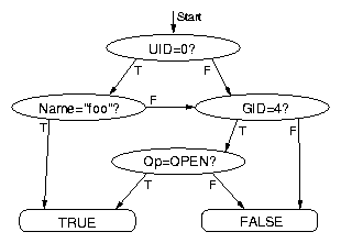
 { cuid = 0 OR cgid = 1 }
 { stream = { STR_POST_OP | STR_PID | STR_UID | STR_TIMESTAMP } }
 { compress; filename = "/mnt/trace.log" buf = 262144 }
}

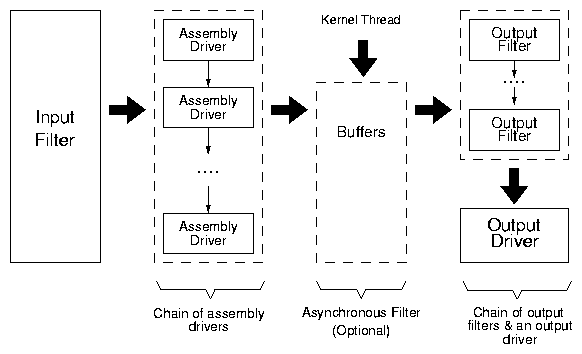
The configuration file contains three sections for each tracer: input filter, assembly drivers, and output filters and driver. In this example, the input filter contains two OR-ed predicates. It uses the stream assembly driver, with the parenthesized parameters specifying the verbosity settings. 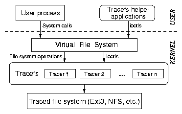Finally, the output chain consists of the compression filter and the file output driver that specifies the name of the trace file and the buffer size being used. This configuration file is parsed by a tool that calls ioctls to specify the tracer. For the input filter, the tool first constructs a DAG which is then passed to the kernel in a topologically-sorted array. The kernel reconstructs the DAG from this array. If the trace parameters are correct, the kernel returns a unique identifier for the tracer. This identifier can be used later to start and stop tracing using ioctls.

The input filter determines which operations will be traced and under what conditions. The ability to limit traces provides flexibility in applying Tracefs for a large variety of applications. We now discuss three such applications: trace studies, IDSs, and debugging.

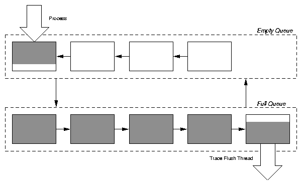
Trace Studies When configuring Tracefs for collecting traces for studies, typically all operations will be traced using a simple or null input filter. The stream assembly driver will trace all arguments. The output driver will typically be a file with buffered asynchronous writes for maximum performance.

For trace studies that involve analysis of the distribution of file-system operations and their timing, the aggregate assembly driver can be used in conjunction with a simple or null input filter. The aggregate driver provides detailed information about operations with minimal overhead. For example, using the aggregate driver, it is easy to determine which operations take the longest time, and to locate anomalous behavior, such as a small fraction of write operations taking an abnormally large time to complete. We have used Tracefs to analyze the performance of other file systems during their development.

Intrusion Detection Systems An IDS is configured with two tracers. The first tracer is an aggregate counter that keeps track of how often each operation is executed. This information is periodically updated and a monitoring application can raise an alarm in case of abnormal behavior. The second tracer creates a detailed operation log. In case of an alarm, the IDS can read this log and get detailed information of file system activity. An IDS needs to trace only a few operations. The output filter includes checksumming and encryption for security. The trace output is sent over a socket to a remote destination, or written to a non-erasable tape. Additionally, compression may be used to limit network traffic.

To defeat denial of service attacks, a QoS output filter can be implemented. Such a filter can effectively throttle file system operations, thus limiting resource usage.

Debugging For debugging file systems, Tracefs can be used with a precise input filter, which defines only the operations that are a part of a sequence of operations known to be buggy. Additionally, specific fields of file system objects can be traced, (e.g., the inode number, link count, dentry name, etc.). No output filters need to be used because security and storage space are not the primary concern and the trace file should be easy to parse. The file output driver is used in unbuffered synchronous mode to keep the trace output as up-to-date as possible.

Chapter 3
Implementation

We developed a prototype of Tracefs as a kernel module for Linux 2.4.20 based on a stackable file system template [22]. Tracefs is 9,272 lines of code. The original stacking template was 3,659 lines of code. The netlink socket output driver is not yet implemented.

We now describe three interesting aspects of our implementation: system-call based filtering, file-name based filtering and asynchronous filter.

3.1 System call based filtering

To support system call based filtering, we needed to determine which system call invoked the file system operation. System call numbers are lost at the file system level. All other information that we log is available either through function parameters, or globally (e.g., the current running task structure contains the PID, current UID, etc.). System call filtering requires a small patch to the kernel. The patch is required only for this additional functionality. All other features are still available without any modifications to the Linux kernel.

We added an extra field, sys_call, to struct task_struct, the structure for tasks. All system calls are invoked through a common entry point parameterized by the system call number. We added four lines of assembly code to the system call invocation path to set the system call number in the task structure before entry and then reset it on exit. In Tracefs, we can filter based on the system call number by comparing the sys_call field of the current process's task structure with a bitmap of system calls being traced. We can also record the system call number for each operation so that file system operations can be correlated with system calls.

3.2 File name based filtering

Implementation of file name based filtering posed a challenge when developing Tracefs. The name of the file is available only in the dentry object of a file, not in the inode. There are some VFS operations that do not pass the dentry object to the file system. Even in cases when the dentry is available, comparison of file names might require expensive string matching.

To implement file name and file extension based tracing, we developed a file name cache that stores all inode numbers for inodes that match a specified name or extension. In case of hard links, the inode number is present in every name group that the names of the file satisfy.

Figure 3.1: The file name cache for tracing based on file names and extensions. The first level table maps a name to an inode number table that stores inode numbers with that name. An input filter has a direct reference to the inode number table.

Figure 3.1 shows the structure of the name cache. The figure shows that the name cache is implemented as a two-level hash table. The first level table maps the name or extension to a second level table that stores all the inode numbers that satisfy the rule. The input filter has a direct reference to an inode table. A file name predicate is evaluated by simply looking up the inode number in the inode table. We create a new entry in the table for a newly created inode if its name satisfies any of the rules; the entry is removed when the inode is flushed from memory. Multiple input filters share the same inode table if they are evaluating the same file name predicate. In the figure, foo.tex is one of the file names being traced. This will trace operations on all files named foo.tex. The entry in the first level table for foo.tex points to an inode table that contains three entries, one for each inode that has the name foo.tex. The input filter that has a file name predicate for foo.tex directly refers to the inode table for predicate evaluation.

3.3 Asynchronous filter

The asynchronous filter allows Tracefs to move expensive operations out of the critical execution path, as described in Section 2.4. Figure 3.2 shows the structure of the asynchronous filter. The filter maintains a list of buffers and two queues: the empty queue and the full queue. The empty queue contains the list of buffers that are currently free and available for use. The full queue contains buffers that are filled and need to be written out. The buffer size and the number of buffers can be configuring during trace setup.

Figure 3.2: The asynchronous filter for performing stream transformations asynchronously. A separate kernel thread is used to transform the stream and write traces to stable storage.

The main execution thread picks the first available buffer from the empty queue and makes it the current buffer. The trace stream is written into this current buffer until it is filled up, at which point it is appended to the full queue and the next empty buffer is picked up. A separate kernel thread is spawned at tracing startup; it gets a buffer from the full queue, writes the buffer to the next output filter, and inserts the emptied-out buffer into the empty queue. Each queue has a counting semaphore that indicates the number of buffers available in it. Both threads wait on the respective queue semaphores when they are zero.

Chapter 4
Evaluation

We evaluated the performance of Tracefs on a 1.7GHz Pentium 4 machine with 1.2GB of RAM. All experiments were conducted on a 30GB 7200 RPM Western Digital Caviar IDE disk formatted with Ext3. To isolate performance characteristics, the traces were written to a separate 10GB 5400 RPM Seagate IDE disk. To reduce ZCAV effects, the tests took place in a separate partition toward the outside of the disk, and the partition size was just large enough to accommodate the test data [8]. The machine ran Red Hat Linux 9 with a vanilla 2.4.20 kernel. Our kernel was modified with a patch for tracing by system call number, so that we could include system call numbers in the trace. However, the results obtained without the optional kernel patch were indistinguishable from those we discuss here. To ensure cold cache, between each test we unmounted the file system on which the experiments took place and to which the traces were written. All other executables and libraries (e.g., compilers) were located on the root file system. We ran all tests at least ten times, and computed 95% confidence intervals for the mean elapsed, system, and user times using the Student-t distribution. In each case, the half-width of the interval was less than 5% of the mean.

4.1 Configurations

Tracefs can be used with multiple different configurations. In our benchmarks, we chose indicative configurations to evaluate performance over the entire spectrum of available features. We conducted the tests at the highest verbosity level of the stream assembly driver so that we could evaluate worst case performance. We selected seven configurations to isolate performance overheads of each output filter and output driver:

EXT3: A vanilla Ext3, which serves as a baseline for performance of other configurations.

FILE: Tracefs configured to generate output directly to a file using a 256KB buffer for traces. We chose a buffer size of 256KB instead of the default of 4KB because our experiments indicated that a 256KB buffer improves the performance on our test setup by 4-5% over 4KB and there are no additional gains in performance with a larger buffer.

UNBUFFERED-FILE: Tracefs configured to generate output to a file without using internal buffering.

CKSUM-FILE: Tracing with an HMAC-MD5 digest of blocks of 4KB, followed by output to a file.

ENCR-FILE: Blowfish cipher in CBC mode with 128-bit keys, followed by output to a file. We used Blowfish because it is efficient, well understood, and was designed for software encryption [20].

COMPR-FILE: Tracing with zlib compression in default compression mode, followed by output to a file.

CKSUM-COMPR-ENCR-FILE: Tracing with checksum calculation followed by compression, then encryption, and finally output to a file. This represents a worst-case configuration.

We also performed experiments for tracing different operations. This demonstrates the performance with respect to the rate of trace generation. We used the aggregate driver to determine the distribution of file system operations and chose a combination of file system operations that produces a trace whose size is a specific fraction of the full-size trace generated when all operations are traced. We used the following three configurations:

FULL: Tracing all file system operations.

MEDIUM: Tracing only the operations that comprise 40-50% of a typical trace. Our tests with the aggregate driver indicated that open, close, read, write, create, and unlink form 40-50% of all trace messages. We chose these operations because they are usually recorded in all studies. Roselli's study also shows that these operations form 49.5% of all operations [19].

LIGHT: Tracing only the operations that comprise approximately 10% of a typical trace. We chose open, close, read, and write for this configuration based on the results of our test. This configuration generates traces with an order of magnitude fewer operations than for FULL tracing.

To determine the computational overhead of evaluating input filters, we executed a CPU-intensive benchmark with expressions of various degrees of complexity, containing 1, 10, and 50 predicates. A one-predicate expression is the simplest configuration and demonstrates the minimum overhead of expression evaluation. We believe that practical applications of tracing will typically use expressions of up to ten predicates. We used 50 predicates to demonstrate worst case performance. The expressions were constructed so that the final value of the expression can be determined only after all predicates are evaluated.

4.2 Workloads

We tested our configurations using two workloads: one CPU intensive and the other I/O intensive. We chose one benchmark of each type so that we could evaluate the performance under different system activity levels. Tracing typically results in large I/O activity. At the same time, our output filters perform CPU-intensive computations like encryption and compression. The first workload was a build of Am-Utils [16]. We used Am-Utils 6.1b3, which contains 430 files and over 60,000 lines of C code. The build process begins by running several hundred small configuration tests to detect system features. It then builds a shared library, ten binaries, four scripts, and documentation. The Am-Utils build process is CPU intensive, but it also exercises the file system because it creates a large number of temporary files and object files. We ran this benchmark with all of the configurations mentioned in Section 4.1.

The second workload we chose was Postmark [10]. We configured Postmark to create 20,000 files (between 512 bytes and 10KB) and perform 200,000 transactions in 200 directories. This benchmark uses little CPU, but is I/O intensive. Postmark focuses on stressing the file system by performing a series of file system operations such as directory lookups, creations, and deletions. A large number of small files being randomly modified by multiple users is common in electronic mail and news servers [10].

4.3 Am-Utils Results

Figure 4.1 shows the results of the Am-Utils build. The figure depicts system, user, and elapsed times for Am-Utils under different configurations of Tracefs. Each bar shows user time stacked over the system time. The height of the bar depicts the total elapsed time for execution. The error bars show the 95% confidence interval for the test. Each group of bars shows execution times for a particular configuration of output filters and output drivers while bars within a group show times for LIGHT, MEDIUM, and FULL tracing. The leftmost bar in each group shows the execution time on Ext3 for reference.

Figure 4.1: Execution times for an Am-Utils build. Each group of bars represents an output filter configuration under LIGHT, MEDIUM, and FULL tracing. The leftmost bar in each group shows the execution time for Ext3.

Tracefs incurs a 1.7% elapsed time overhead for FULL tracing when tracing to a file without any output filters. Checksum calculation and encryption introduce additional overheads of 0.7% and 1.3% in elapsed time. Compression results in 2.7% elapsed time overhead. Combining all output filters results in a 5.3% overhead. System time overheads are 9.6-26.8%. The base overhead of 9.6% is due to stacking and handling of the trace stream. CPU intensive stream transformations introduce additional overheads. The low elapsed time overheads indicate that users will not notice a change in performance under normal working conditions.

Under MEDIUM workload, Tracefs incurs a 1.1% overhead in elapsed time when writing directly to a trace file. Checksum calculation and encryption have an additional overhead of less than 1%. Compression has an additional 2.3% overhead. The system time overheads vary from 7.6-13.7%.

Finally, under LIGHT workload, Tracefs incurs less than 1% overhead in elapsed time. The output filters result in an additional overhead of up to 1.1%. System time overheads vary from 6.1-8.6%.

Unbuffered I/O with FULL tracing has an overhead of 2.7%. The system time overhead is 13.7%, an increase of 4.1% over buffered I/O. This shows that buffered I/O provides better performance, as expected.

Overall, these results show that Tracefs has little impact on elapsed time, even with encryption, compression, and checksumming. Among the output filters, compression incurs the highest performance overhead. However, we can see from Figure 4.3 that the trace file shrinks from 51.1MB to 2.7MB, a compression ratio of 18.8. This indicates that compression is useful for cases where disk space or network bandwidth are limited.

Input Filter Performance We evaluated the performance of input filters on the Am-Utils workload because it is CPU intensive and it gives us an indication of the CPU time spent evaluating expressions under a workload that already has high CPU usage. We tested with input filters containing 1, 10, and 50 predicates. We considered two cases: a FALSE filter that always evaluates to false, and thus never records any trace data; and a TRUE filter that always evaluates to true, and thus constructs the trace data, but writes it to /dev/null.

With a FALSE one-predicate input filter, the system time overhead is 4.5%; with a TRUE filter, the overhead is 11.0%. For a ten-predicate input filter, the system time overhead is 8.7% for a false expression and 12.6% for a true expression. Going up to a fifty-predicate filter, the overhead is 16.1% for a FALSE filter and 21.8% for a TRUE filter. In terms of elapsed time, the maximum overhead is 4% with a fifty-predicate filter. Therefore, we can see that Tracefs scales well with complex expressions, and justifies our use of directed acyclic graphs for expression evaluation, as described in Section 2.2.

4.4 Postmark Results

Figure 4.2 shows the execution times for Postmark. This figure has the same structure as Figure 4.1 and shows results for the same Tracefs configurations for Postmark.

Figure 4.2: Execution times for Postmark. Each group of bars represents an output filter configuration under LIGHT, MEDIUM, and FULL tracing. The leftmost bar in each group shows execution times for Ext3.

The figure shows that Tracefs incurs 12.4% overhead in elapsed time for FULL tracing. Encryption introduces another 3.7% overhead, and checksum calculation has an additional overhead of 2.8%. Compression has an overhead of 6.1% in elapsed time. The system time overheads are higher: 132.9% without any output filters, whereas encryption, checksum calculation, and compression have additional overheads of 80.4%, 36.9%, and 291.4%, respectively. However, Figure 4.2 shows that system time is a small portion of this I/O-intensive benchmark and the performance in terms of elapsed time is reasonable considering the I/O intensive nature of the benchmark.

For MEDIUM tracing, the elapsed time overhead is 10.0%. Encryption, checksum calculation, and compression have additional elapsed time overheads of 2.2%, 0.9%, and 5.2%, respectively. The system time increases by 90.6% without any output filters; encryption, checksum calculation, and compression have additional overheads of 28.7%, 12.8%, and 140.7%, respectively. LIGHT tracing has an overhead ranging from 5.9-11.3% in elapsed time. System time overheads vary from 70.1-122.8%. This shows that selective tracing can effectively limit the computational overheads of transformations. Reducing the trace configuration from FULL to MEDIUM tracing reduces the system time overhead by a factor of 2.1. From FULL to LIGHT tracing, the system time overhead is reduced by a factor of 3.4.

Input Filter Performance We evaluated the performance of input filters for the Postmark workload using a worst-case configuration: a 50-predicate input filter that always evaluates to true, in conjunction with the CKSUM-COMPR-ENCR-FILE configuration of output filters and with FULL tracing. In this configuration, the elapsed time increases from 767 to 780 seconds, an increase of 1.7%, as compared to a one-predicate input filter. This is less than the overhead for Am-Utils because Postmark is I/O intensive.

4.5 Trace File Sizes and Creation Rates

Figure 4.3 shows the size of trace files (left half) and the file creation rates (right half) for the Am-Utils and Postmark benchmarks. Each bar shows values for FULL, MEDIUM, and LIGHT tracing under a particular configuration. The bar for FILE also shows variation in file size (and rate) for CKSUM-FILE and ENCR-FILE configurations; the values for these two configurations were similar and we excluded them for brevity.

Figure 4.3: Trace file sizes and creation rates for Postmark and Am-Utils benchmarks. Each bar shows values for FULL, MEDIUM, and LIGHT tracing. The left half depicts file sizes and the right half depicts trace file creation rates

This figure shows that Postmark generates traces at a rate 2.5 times faster than an Am-Utils build. This explains the disparity in overheads between the two benchmarks. Encryption does not increase the file size whereas checksumming increases the file size marginally because checksums are added to each block of data. Trace files achieve a compression ratio in the range of 8-21. The file creation rate decreases as output filters are introduced. However, the rate shows an increase from COMPR-FILE to CKSUM-COMPR-ENCR-FILE since the file size increases because of checksum calculation. The figure also demonstrates how trace files can be effectively reduced in size using input filters.

4.6 Effect of Asynchronous Writes

There are two aspects to Tracefs's performance with respect to asynchronous writes: (1) writing the trace file to disk, and (2) using the asynchronous filter to perform output filter transformations asynchronously.

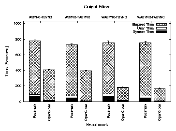
	Synchronous File System	Asynchronous Filter
WSYNC-TSYNC	yes	no
WSYNC-TASYNC	yes	yes
WASYNC-TSYNC	no	no
WASYNC-TASYNC	no	yes

Table 4.1: File system and asynchronous filter configurations for evaluating the performance of the asynchronous filter.

Table 4.1 lists the four different configurations of the asynchronous filter used for the evaluation. All benchmarks mentioned previously were performed in WASYNC-TSYNC mode since it is the default configuration for Tracefs and the file system to which the traces were written (Ext2/3). To study the effects of asynchronous writes, we performed two benchmarks: (1) Postmark with a configuration as mentioned in Section 4.2, and (2) OpenClose, a micro-benchmark that performs open and close on a file in a tight loop using ten threads, each thread performing 300,000 open-close pairs. We chose OpenClose since we determined that general-purpose benchmarks like Postmark perform large I/O on the underlying file system but produce comparatively little I/O for tracing. The OpenClose micro-benchmark is designed to generate large trace data without writing much data to the underlying file system.

Figure 4.4: Execution times for Postmark and OpenClose. Bars show system, user, and elapsed times for all combinations of asynchronous filter and trace file writes.

Figure 4.4 shows the system, user, and elapsed times for the two benchmarks under the four configurations. Elapsed time Postmark increases by 3.0% when the traces were written synchronously as compared to asynchronous writes; such an all-synchronous mode is useful for debugging or security applications. For the intensive OpenClose benchmark, synchronous disk writes increase the elapsed time by a factor of 2.3.

The asynchronous filter lowers the elapsed time for execution of Postmark by 6.0% with synchronous trace file writes. The change with asynchronous disk writes is negligible. For OpenClose, the elapsed time reduces by 3.9% with synchronous disk writes and 7.5% with asynchronous disk writes. The larger improvement is the result of the micro-benchmark stressing the tracing subsystem by generating large traces without actual I/O. The asynchronous filter is useful in such cases.

4.7 Multi-Process Scalability

We evaluated the scalability of Tracefs by executing multiple Postmark processes simultaneously. We configured Postmark to create 10,000 files (between 512 bytes and 10KB) and perform 100,000 transactions in 100 directories for one process, but the workload was evenly divided among the processes by dividing the number of files, transactions, and subdirectories by the number of processes. This ensures that the number of files per directory remains the same. We measured the elapsed time as the maximum of all processes, because this is the amount of time that the work took to complete. We measured the user and system time as the total of the user and system for each process. We executed the benchmark in the FILE configuration with FULL tracing for 1, 2, 4, 8, and 16 processes.

Figure 4.5: Elapsed and system times for Postmark with Ext3 and Tracefs with multiple processes

Figure 4.5 shows the elapsed and system times for Postmark with multiple processes. With a single process, the elapsed time is 383 seconds on Ext3 and 444 seconds with Tracefs. For 16 processes, the elapsed time reduces by a factor of 5.6 on Ext3 and by a factor of 3.3 with Tracefs. This shows that Tracefs scales well with multiple processes, though by a lesser factor, as compared to Ext3. This can be attributed to the serialization of writing traces to disk. The system times remain constant for both Ext3 and Tracefs.

4.8 Anonymization Results

Anonymization tests were conducted by anonymizing selected fields of a trace file generated during one run of our Postmark benchmarks under FULL tracing with no output filters. We chose the following five configurations for anonymization:

Null anonymization. The trace is parsed and rewritten. This serves as the baseline for comparison.
Process name, file name, and strings anonymized. This accounts for 12.5% of the trace.
UIDs and GIDs anonymized. This accounts for 17.9% of the trace file.
Process names, file names, UIDs, GIDs, and strings anonymized. This accounts for 30.4% of the trace.
Process names, file names, UIDs, GIDs, PIDs and strings anonymized. This accounts for 39.3% of the trace.
Process names, file names, UIDs, GIDs, PIDs, strings, and timestamps anonymized. This accounts for 48.2% of the trace.

Figure 4.6 shows the performance of our user-level anonymization tool. The figure shows the size of the anonymized traces in comparison to the original trace file as bars. It also shows the rate of anonymization as a line. The rate of anonymization is the rate at which the unanonymized input trace file can be processed by the anonymization tool.

The leftmost bar in the figure shows the base configuration where no data is anonymized. Each bar shows the size of the anonymized file and the increase in size over the original file. The line shows the rate of anonymization in KBps. The base configuration shows the rate of parsing without any anonymization.

Figure 4.6: Trace file anonymization rates and increase in file sizes for different portions of traces anonymized. The Y₁ axis shows the scale for file sizes whereas the Y₂ axis shows the scale for the rate of anonymization.

In the figure we see that the rate of anonymization decreases as a larger percentage of data is anonymized, as expected. The rate of anonymization decreases by 30.5% whereas the percentage of anonymized data is increased by 48.2%. The rate of anonymization is limited by the increased I/O required for larger trace files. Anonymization increases the trace file size since fields in the trace need to be padded up to the encryption block size. Also, anonymized constant-length fields are converted into variable-length fields since anonymization changes the length of the field. The length of variable-length fields needs to be stored in the trace.

In summary, we evaluated Tracefs's performance using CPU-intensive and I/O-intensive benchmarks under different configurations, and show that Tracefs has acceptable overheads under normal conditions, even with CPU-intensive output filters, or complex input filters.

Chapter 5
Related Work

In this section we discuss six past trace studies and systems that motivated our design.

File System Tracing Package for Berkeley UNIX

In 1984, Zhou et al. implemented a tracing package for the UNIX file system [23]. They instrumented the file operations and process-control-related system calls to log the call and its parameters. Their traces are collected in a binary format and buffered in the kernel before writing to the disk. The package uses a ring of buffers that are written asynchronously using a user-level daemon. The tracing system also switches between trace files so that primary storage can be freed by moving the traces to a tape. The generated binary traces are parsed and correlated into open-close sessions for study. The overhead of tracing is reported up to 10%. The package is comprehensive: it allows tracing of a large number of system calls and logs detailed information about the parameters of each call. However, it provides little flexibility in choosing which calls to trace and the verbosity of the trace. The generated traces require laborious post-processing. Finally, tracing at the system call level makes it impossible to log memory-mapped I/O or to trace network file systems.

BSD Study

In 1985, Ousterhout et al. implemented a system for analyzing the UNIX 4.2 BSD file system [15]. In this study, they traced three servers over a period of 2-3 days. This system was implemented by modifying the BSD kernel to trap file-system-related system calls. They chose not to trace reads or writes to avoid generating large traces and consuming too much CPU. Memory-mapped I/O was estimated by logging execve. The BSD study was one of the first file system studies and its results influenced the design of future file systems. However, the tracing system used in the study is too specific to be used for other applications. The system traced few operations and other file system activity was inferred, rather than logged. Important file system operations like read, write, lookup, directory reads, and accessing file inodes were not considered.

Sprite Study

In 1991, Baker et al. conducted a study on user-level file access patterns on the Sprite operating system [1]. They studied file system activity for the Sprite distributed file system served by four file servers, over four 48-hour periods. In this study, they repeated the analysis of the BSD study. They also analyzed file caching in the Sprite system. They instrumented the Sprite kernel to trace file system calls and periodically feed the data to a user-level logging process. Cache performance was studied by using counters in the kernel that were periodically retrieved and stored by a user-level program. The use of counters provides a light-weight mechanism for statistical evaluation, and we have made similar provisions for aggregate counters in our Tracefs design. However, the Sprite traces are limited to a few file system operations. Like the BSD study, the Sprite study did not record read and write operations to limit CPU and storage overheads. In comparison, Tracefs provides a flexible mechanism to selectively trace any set of file system operations.

Windows NT 4.0 Study

In 1998, Vogels conducted a usage study on the Windows NT file system [21]. The purpose of this study was to conduct BSD and Sprite like studies, in the context of changes in computing needs. The usage of components of the Windows NT I/O subsystem was studied. The study was conducted on a set of 45 systems in distinct usage environments. Traces were collected by using a filter driver that intercepts file system requests. The trace driver records 54 I/O request packet (IRP) events on local and remote file system activity covering all major I/O operations. Memory-mapped I/O was also traced. Due to the nature of Windows NT paging, separating actual file system operations from the other VM activity is difficult and must be done during post-processing. This VM activity almost doubled the size of the traces. Also, daily snapshots of local file systems were taken to record the file system hierarchy. Traces were logged to a remote collection server, and analyzed using data-warehousing techniques.

Roselli Study

In 2000, Roselli et al. collected and analyzed file system traces from four separate environments running HP-UX 9.05 and Windows NT 4.0 [19]. HP-UX traces were collected by using the auditing subsystem to record file system events. Additional changes to the kernel were required to trace changes to the current working directory for resolving relative paths in system calls to absolute pathnames. The use of the auditing subsystem provides a mechanism for selectively tracing file system events with minimal changes to kernel code. The system demonstrates that processes frequently use memory mapped I/O; however, tracing of system calls on Unix makes it impossible to determine paging activity that results either from explicit memory-mapped I/O or from loading of executables. Windows NT traces were collected by interposing file system calls using a file system filter driver. Unfortunately, to collect information on memory-mapped operations they needed to interpose not only file system operations, but also system calls. Roselli's filter driver also suffers from problems related to paging activity that are similar to Vogels's.

Passive Network Monitoring

Passive network monitoring has been widely used to trace activity on network file systems. Passive tracing is performed by placing a monitoring system on the network that snoops all NFS traffic. The captured packets are converted into a human-readable format and written to a trace file. Post-processing tools are used to parse the trace file and correlate the RPC messages.

Blaze implemented two tools, rpcspy and nfstrace, to decode RPC messages and analyze NFS operations by deriving the structure of the file system from NFS commands and responses [2].

Ellard et al. implemented a set of tools for anonymization and analysis of NFS traces. These tools capture NFS packets and dump the output in a convenient human-readable format [5,7]. The traces are generated in a table format that can be parsed using scripts and analyzed with spreadsheets and database software.

Passive tracing has the advantage of incurring no overhead on the traced system. It does not require any modifications to the kernel and can be applied to trace any system that supports the NFS protocol. It also enables the study of an NFS based system as a whole, which is not possible through system call based kernel instrumentation strategies [13,14]. However, NFS traces are not fully accurate since network packets can be dropped or missed. Passive tracing also does not provide accurate timing information. The NFSv2 and NFSv3 protocols do not have open and close commands which make it impossible to determine file access sessions accurately. Memory-mapped I/O cannot be distinguished from normal reads and writes using passive NFS tracing. Passive tracing also does not provide an easy mechanism for capturing specific data; large amounts of traces need to be captured and analyzed during post-processing to extract specific information.

Tracefs can be used for monitoring the file system at the server since the tracing is performed at the file system level instead of system call level. Tracefs provides fine-grained control over the specific data to be traced which makes post-processing easier.

Chapter 6
Conclusions

Our work has three contributions. First, we have created a low-overhead and flexible tracing file system that intercepts operations at the VFS level. Unlike system call tracing, file system tracing records memory-mapped operations. Unlike NFS tracing, file system tracing receives open and close events. For normal user operations, even with the most verbose traces, our overhead is less than 2%. Our system has several modular components: assembly drivers provide different trace formats or aggregate statistics; output filters perform transformations on the data (e.g., compression or encryption); and output drivers write the traces to various types of media. Low overhead and flexibility makes Tracefs useful for applications where tracing was previously unused: file system debugging, intrusion detection, and more.

Second, Tracefs supports complex input filters that can reduce the amount of trace data generated. Using an input filter to capture open, close, read, and write events, an I/O-intensive workload has only a 6% overhead. Input filters also increase Tracefs's usefulness as a security tool. Tracefs can intercept only suspicious activity and feed it to an IDS.

Third, our trace format is self-contained. No additional information aside from the syntax is required to parse and analyze it. Our trace contains information about the machine that was being traced (memory, processors, disks, etc.) as well as OS information. Rather than use embedded numbers with special meaning, our traces contain mappings of numbers to plaintext operations to ease further analysis (e.g., all system call numbers are recorded at the beginning of the trace).

6.1 Future Work

Our main research focus in this project now shifts to support replaying traces, including selective trace replaying, and replaying at faster or slower rates than the original trace. Replaying traces is useful for several reasons. First, to be able to repeat a sequence of file system operations under different system conditions (e.g., evaluating with a new file system). Second, for debugging, it is especially useful for validating the reproducibility of a bug in file system code or for changing timing conditions when tracking down a race-condition. Third, for computer forensics it is useful to be able to go back and forth in a trace of suspicious activity, inspecting actions in detail. To support flexible trace replaying, we are investigating what initial state information needs to be recorded in the traces, and possible trace format enhancements.

We are also exploring a few additional aspects of Tracefs. First, we would like to provide a tool to convert binary traces into XML, which can then be processed easily by XML parsers. Second, we are investigating support for capturing lower level disk block information. This information is useful for file system developers to determine optimal on-disk layout. This information is not easily available in a stackable file system.

Bibliography

[1]: M. G. Baker, J. H. Hartman, M. D. Kupfer, K. W. Shirriff, and J. K. Ousterhout. Measurements of a Distributed File System. In Proceedings of 13th ACM Symposium on Operating Systems Principles, pages 198-212. Association for Computing Machinery SIGOPS, 1991.
[2]: M. Blaze. NFS Tracing by Passive Network Monitoring. In Proceedings of the USENIX Winter Conference, January 1992.
[3]: D. J. Brown and K. Runge. Library interface versioning in solaris and linux. In Proceedings of the Annual Linux Showcase and Conference, October 2000.
[4]: P. Deutsch and J. L. Gailly. RFC 1050: Zlib 3.3 Specification. Network Working Group, May 1996.
[5]: D. Ellard, J. Ledlie, P. Malkani, and M. Seltzer. Passive NFS Tracing of Email and Research Workloads. In Proceedings of the Annual USENIX Conference on File and Storage Technologies, March 2003.
[6]: D. Ellard, J. Ledlie, and M. Seltzer. The Utility of File Names. Technical Report TR-05-03, Computer Science Group, Harvard University, March 2003.
[7]: D. Ellard and M. Seltzer. New NFS Tracing Tools and Techniques for System Analysis. In Proceedings of the Annual USENIX Conference on Large Installation Systems Administration, October 2003.
[8]: D. Ellard and M. Seltzer. NFS Tricks and Benchmarking Traps. In Proceedings of the Annual USENIX Technical Conference, FREENIX Track, pages 101-114, June 2003.
[9]: LBNL Network Research Group. The TCPDump/Libpcap site. www.tcpdump.org, February 2003.
[10]: J. Katcher. PostMark: A New Filesystem Benchmark. Technical Report TR3022, Network Appliance, 1997. www.netapp.com/tech_library/3022.html.
[11]: G. H. Kuenning. Seer: Predictive File Hoarding for Disconnected Mobile Operation. PhD thesis, University of California, Los Angeles, May 1997.
[12]: S. McCanne and V. Jacobson. The BSD Packet Filter: A New Architecture for User-level Packet Capture. In Proceedings of the Winter USENIX Technical Conference, pages 259-69, January 1993.
[13]: A. W. Moore. Operating system and file system monitoring: A comparison of passive network monitoring with full kernel instrumentation techniques. Master's thesis, Department of Robotics and Digital Technology, Monash University, 1998.
[14]: A. W. Moore, A. J. McGregor, and J. W. Breen. A comparison of system monitoring methods, passive network monitoring and kernel instrumentation. ACM SIGOPS Operating Systems Review, 30(1):16-38, 1996.
[15]: J. Ousterhout, H. Costa, D. Harrison, J. Kunze, M. Kupfer, and J. Thompson. A Trace-Driven Analysis of the UNIX 4.2 BSD File System. In Proceedings of the Tenth ACM Symposium on Operating System Principles, pages 15-24, Orcas Island, WA, December 1985. ACM.
[16]: J. S. Pendry, N. Williams, and E. Zadok. Am-utils User Manual, 6.1b3 edition, July 2003. www.am-utils.org.
[17]: H. V. Riedel. The GNU/Linux CryptoAPI site. www.kerneli.org, August 2003.
[18]: R. L. Rivest. RFC 1321: The MD5 Message-Digest Algorithm. In Internet Activities Board. Internet Activities Board, April 1992.
[19]: D. Roselli, J. R. Lorch, and T. E. Anderson. A Comparison of File System Workloads. In Proc. of the Annual USENIX Technical Conference, pages 41-54, June 2000.
[20]: B. Schneier. Applied Cryptography. John Wiley & Sons, second edition, October 1995.
[21]: W. Vogels. File System Usage in Windows NT 4.0. In Proceedings of the 17th ACM Symposium on Operating Systems Principles, pages 93-109, December 1999.
[22]: E. Zadok and J. Nieh. FiST: A Language for Stackable File Systems. In Proceedings of the Annual USENIX Technical Conference, pages 55-70, June 2000.
[23]: S. Zhou, H. Da Costa, and A. J. Smith. A File System Tracing Package for Berkeley UNIX. In Proceedings of the USENIX Summer Conference, pages 407-419, June 1984.
[24]: N. Zhu, J. Chen, T. Chiueh, and D. Ellard. An NFS Trace Player for File System Evaluation. Technical Report TR-14-03, Harvard University, December 2003.

File translated from T_EX by T_TH, version 3.61.
On 30 Aug 2004, 15:21.