Figure 8.3
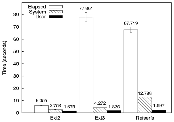
Figure 8.1 shows a simple bar graph with three components and three series (sets of bars). To create this graph, the following command was used:
     graphit --mode=bar --graphfile=pm.eps \
             --components=Elapsed,User,System \
             -f 20 \
             --ylabel "Time (seconds)" \
             'Ext2' ext2/ext2:1.res \
             'Ext3' ext3/ext3:1.res \
             'Reiserfs' reiserfs/reiserfs:1.res
The first line informs graphit that we are creating a bar graph that should be output to pm.eps. The second line indicates that each set of bars, should have Elapsed, User, and System time components. The third line increases the font size to 20 points. The fourth line sets the y-axis label to Time (seconds). Lines 5–7 define the series. Ext2 is taken directly from the results file ext2/ext2:1.res, Ext3 is taken from ext3/ext3:1.res, etc.
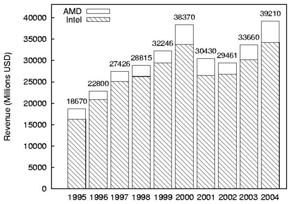
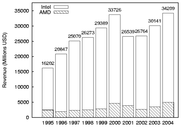
Bar graphs can also be generated from CSV files. fig:revenue-nostack is a bar graph generated from the following CSV file containing revenue (in Millions of US dollars) for AMD and Intel:
     Year,AMD,Intel
     1995,2468,16202
     1996,1953,20847
     1997,2356,25070
     1998,2542,26273
     1999,2857,29389
     2000,4644,33726
     2001,3891,26539
     2002,2697,26764
     2003,3519,30141
     2004,5001,34209
The command line to generate this graph was:
     graphit --mode=bar --graphfile=revenue.eps \
             --ylabel "Revenue (Millions USD)" -f 20 \
             --components=AMD,Intel \
             '[0-9]*' revenue.csv
The components map to the columns in the CSV file, and Year was
automatically selected for the Series names because there were no other
columns. All of the values in the CSV file were selected, because the
regular expression '[0-9]*' matches all of the years. To graph the only
revenue for 1999-2004, you could use regular expression
(1999|2.*) instead.
Stacked bars are displayed such that the bottom of bar starts at
the top of another bar. In Figure 8.1, User time is stacked on
System time. By default User is stacked over System, but no other bars
are stacked. To disable stacking you can use the --nostack
option. To stack two components specify --stack
Top/Bottom on the Graphit command line.
For example, lets assume we did not want to stack the values in Figure 8.1. We could use a command line like the following:
     graphit --mode=bar --graphfile=pm.eps \
             --components=Elapsed,User,System \
             -f 20 --ylabel "Time (seconds)" \
             --nostack --bargap 0.25 \
             'Ext2' ext2-1/ext2:1.res \
             'Ext3' ext3-2/ext3:1.res \
             'Reiserfs' reiserfs-1/reiserfs:1.res
The only differences with the previous graph are the addition of the --nostack option, and the --bargap 0.25 option. The --bargap option is used to spread the individual bars out. If we did not spread out the bars, then it would be possible for System time to completely cover User time (or vice versa). We specified 0.25 as the gap between bars, because each bar is 0.25 artificial x-units large by default (the default spacing is 0, so each bar in the group lines up precisely with the other bars). The graph produced by this command is shown in fig:nostack.
Figure 8.5 is the same graph as Figure 8.3, but AMD's revenue is stacked on top of Intel's. This type of graph is a better depiction about the total revenue for both companies, because we can visually see the revenue changes, without needing to add them in our head. The labels above each bar on this graph are the total revenue for both AMD and Intel.
The simplest way to create a line graph is to create one based on several results files, like Figure 8.2. To generate this graph, the following command was used:
     graphit --mode=line --graphfile=pm-line.eps \
             --components=Elapsed,System -f 20 \
             --ylabel "Time (seconds)" \
             --xlabel "Threads" \
             Reiserfs 'reiserfs/reiserfs:*.res'\
             Ext3 'ext3/ext3:*.res'
This is rather similar to the command to generate line graphs, but the --mode option is set to line, and instead of a single input file, the input specification specifies a shell globbing pattern. In this case the Reiserfs glob is expanded to reiserfs/reiserfs:1.res, reiserfs/reiserfs:2.res, reiserfs/reiserfs:4.res, reiserfs/reiserfs:8.res, reiserfs/reiserfs:16.res, and reiserfs/reiserfs:32.res. Because reiserfs/reiserfs: is a common prefix, and .res is a common suffix, they are stripped and the x-values are 1, 2, 4, 8, 16, and 32 for each file, respectively.
Line graphs can also be generated from a CSV file. Assume that you have a program that gets faster or slower as it runs. A natural way to show this progression is using a line graph. If you have run the program through Auto-pilot you have a .res file that contains the time for each execution, but you can not directly use it for graphing because Graphit produces one point for a standard results file.
We can use getstats to convert a results file into a CSV file using the following command:
     getstats --nostdtransforms --readpass \
             --rename elapsed Elapsed \
              --rename user User \
             --rename sys System \
             --csv find.res >find.csv
This command skips the standard transformations, performs the
readpass transformation, renames the columns, and produces a
CSV file on stdout, which is redirected to find.csv.
find.csv contains lines like the following
     "epoch","Elapsed","User","System","io","cpu"
     "1","8.231657","0.917859","7.313887","-8.90000000000057e-05","100.001081191794"
     "2","8.647","0.968851","7.264894","0.413255","95.2208280328438"
     ...
Using find.csv, we can generate a graph using the following command:
     graphit --mode=line  --graphfile find.eps \
             --components=Elapsed,User,System
             --xlabel "Run number" --ylabel "Time (seconds)" \
             -Y 10 \
             --Xparser=--xcol=epoch \
             'Find' find.csv
In this example, there are two new options that we used: -Y and
--Xparser. Adding -Y 10 increases the maximum value on
the y-axis to 10, so that the key does not overlap the lines. The
--Xparser=--xcol=epoch option is used to select the column
within the CSV file that is used for X values. We must specify the
--xcol parser option, because there are three possible
candidates (epoch, io, and cpu).